How does Dijkstra's self-stabilizing algorithm work?
System Design practice on Codemia
Work through 120+ system design problems with detailed solutions, from rate limiters to multi-region storage.
Introduction
Self-stabilization is a property of distributed systems that allows them to recover from transient faults, errant data, or arbitrary perturbations, by reaching a legitimate state within finite time without external interventions. Dijkstra's pioneering work on self-stabilization offers a simple yet powerful algorithm that demonstrates how a system can autonomously stabilize, relying purely on localized state transitions. This article delves into Dijkstra's self-stabilizing algorithm, examining its underlying principles, execution, and applicability in distributed systems.
Dijkstra's Self-Stabilizing Algorithm: Overview
Dijkstra's self-stabilizing algorithm addresses the notion of reaching consistency in a ring network, where each node in the network influences its immediate neighbors. The algorithm ensures that no matter the initial states of the nodes, the system eventually reaches a legal configuration and remains so, handling arbitrary state changes locally without any global control.
Key Definitions
- State: The current condition or configuration of a node.
- Configuration: The combined states of all the nodes in a system.
- Legal State: A state deemed correct for a node under certain conditions.
- Configuration Sequence: A sequence representing a series of configurations that a system transitions through.
- Local Rule: A condition that dictates how each node updates its state based on its current state and the state of its neighbors.
Basic Concept
The core premise of the algorithm is to set up a set of rules or conditions for each node such that the system always converges to a legitimate configuration. Each node in the network can determine its state independently by observing its immediate environment (usually adjacent nodes).
Technical Explanations
Network Model
- Topology: Consider a unidirectional ring network consisting of
nnodes, each with a unique identifier. - State Space: Assume each node can be in one of
kstates (typically integers). Notably, Dijkstra used a simplest binary setup in his original proposal (k=2).
System Dynamics
Nodes update their states through a locally defined rule. Let state of node i be denoted as , the global configuration is , and node i can access and . The system can be described by the following conditions:
- Local Rule: Node
iupdates its state if and only if it is not in a legal state. A common rule Dijkstra proposed was:- If , then .
Algorithm Execution
- Initialization: Start with any arbitrary configuration where nodes are in random states.
- State Transition: Nodes observe local rules and update their states whenever applicable.
- Convergence: The system evolves, leading to a legitimate configuration after several iterations.
Example
Imagine a ring with 4 nodes (N_1, N_2, N_3, N_4), each node with states 0 or 1.
Initial Configuration
Iteration Steps
- Configuration 1:
- : No change
- : No change
- : No change
- : Change:
- Configuration 2 (after change):
- New C:
- The process continues until convergence.
Converged Configuration
- Eventually, nodes reach a steady configuration such as , matching the legality condition.
Properties
Self-stabilization Properties
- Convergence: Guaranteed return to a legitimate state within a finite number of steps from any arbitrary initial configuration.
- Closure: Once in a legitimate configuration, the system remains in one barring external disturbances.
Example Applications
Dijkstra's model informs the design of algorithms that require robustness against faults in distributed systems, such as:
- Sensor networks.
- Distributed databases.
- Fault-tolerant computing systems.
Summary
The concise and efficient nature of Dijkstra's self-stabilizing algorithm is summarized below:
| Aspect | Description |
| Network Type | Unidirectional ring topology. |
| Convergence | Achieves stability from any arbitrary state configuration. |
| Locality | Nodes only require state of immediate neighbors to update, ensuring scalability. |
| Applications | Ideal for systems requiring fault tolerance and resilience. |
Dijkstra's algorithm remains an essential concept in distributed computing, offering insights into designing reliable and resilient systems that can autonomously recover from disruptions. Through adaptable local rules, the self-stabilizing approach ensures distributed systems can maintain order, emphasizing localized decision-making for global stability.
Related reading
- How does Distributed Shared Memory work in the presence of cache and registers?
- How does distributed tensorflow work ? Issue with tf.train.Server
- How does Elasticsearch recover from a quorum that is not unanimous
- How does Erlang's support for transparent distribution of actors impact application design?
- How does finding a cycle start node in a cycle linked list work?
- How does Firefox's 'awesome' bar match strings?
- How does etcd propagate writes to non-leader members?
- How does fault tolerance works in a distributed system?
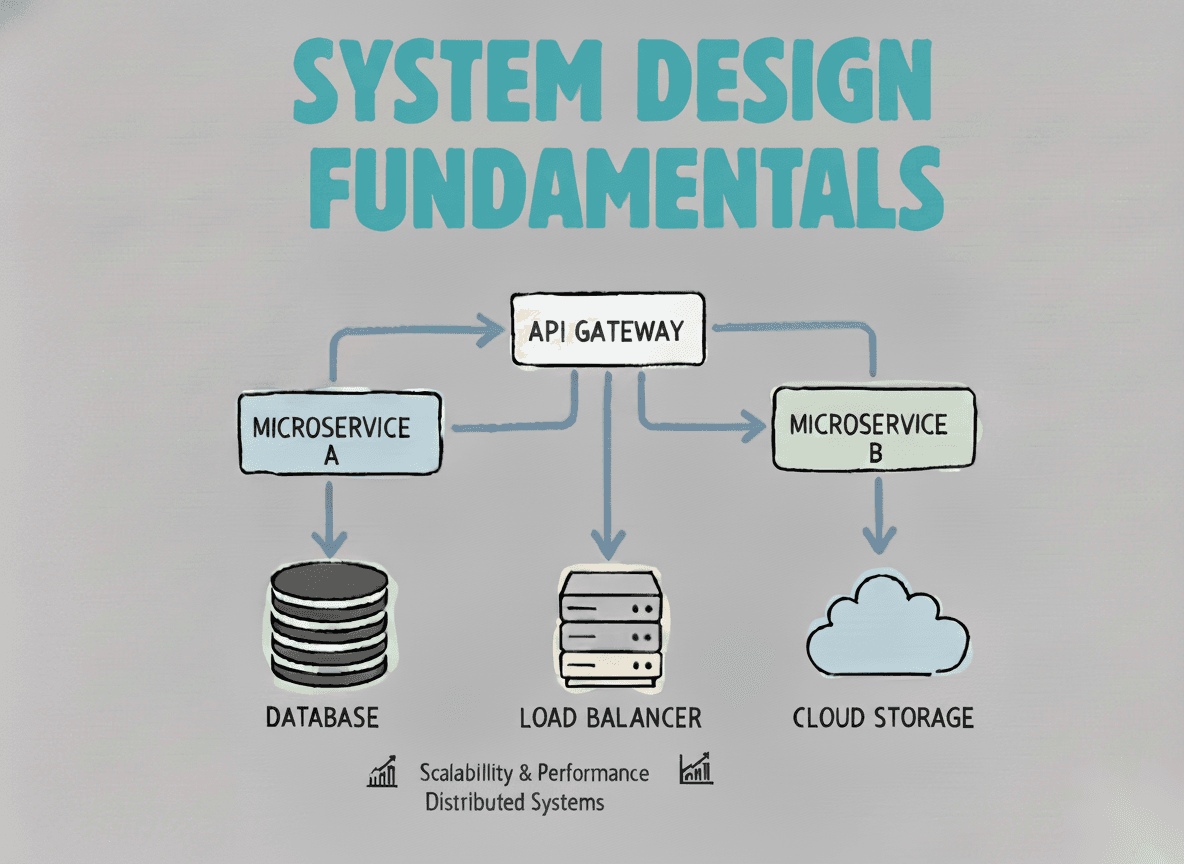
System Design Fundamentals
Build a strong foundation in designing scalable, reliable distributed systems.
View the courseSystem Design practice on Codemia
Work through 120+ system design problems with detailed solutions, from rate limiters to multi-region storage.